Ⅰ. Introduction

The Go competition between the artificial intelligence (AI) AlphaGo of Google DeepMind and the legendary Go player Lee Sedol-in which AlphaGo won 4:1-straightforwardly shows the development of AI. At present, AI is being widely used in

various fields including SPAM mail filters, search algorithms and ranking system of web search engines, facial recognition algorithms of social networking services, and personalized curation algorithms of contents or products (Fig. 1).¹1 Alibaba achieved daily sales $38 billion during the Singles Day in 2019, 26% higher than the previous year, by launching an AI fashion assistant which has been trained about hundreds of millions of clothes. Amazon is automating most of their logistics except packing and is managing “Amazon Go” checkout-free convenience store chain in the US. In the Amazon Go, the payment is automatically processed when customers exit with their products based on real-time location tracking of them using multiple cameras, weight measuring sensors, and deep learning algorithms.

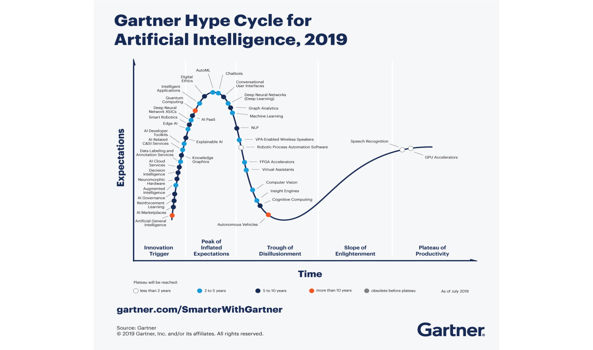
Fig. 1.

Hype cycle for artificial intelligence 2019. Reprinted from “Gartner Hype Cycle for Artificial Intelligence 2019” by Kenneth Brant, Jim Hare, Svetlana Sicular, Copyright 2019 by Gartner, Inc. and/or its affiliates. https://www.gartner.com/smarterwithgartner/top-trends-on-the-gartner-hype-cycle-forartificial-intelligence-2019/

AI is expected to have huge impact on the healthcare industry. Currently, more than 40 and 10 deep learning algorithms have been approved as medical devices by the US Food and Drug Administration (FDA) and Ministry of Food and Drug Safety (MFDS) in South Korea, respectively. For example, fourth-generation Apple Watch and AliveCor KardiaMobile with deep learning algorithm have been approved by the US FDA as over-the-counter medical devices for detecting atrial fibrillation. These algorithms show an accuracy for detecting abnormal findings comparable to that of humans by training hundreds of thousands of data.

Dentistry is a field of study that requires a high level of accuracy; it is expected that AI and deep learning algorithms will be introduced in the near future and provide great assistance to clinical practices. In South Korea, an algorithm that estimates bone age from a hand-wrist radiograph has been approved by the MFDS; however, not many other cases have been reported yet. Therefore, this study aims to examine the global trends of deep learning technologies applied to dentistry and to forecast the future of dentistry.

Ⅱ. Materials and Methods

1. Literature Search

To select literature on the application of deep learning algorithms in dentistry, we searched the MEDLINE and IEEE Xplore databases for papers in all languages that were published before October 24, 2019. The search formula was set up by combining free-text term and entry term about the deep learning, neural network, and dentistry (Table 1).

2. Selection of Papers

Papers were selected in two steps: first, papers were selected based on their title and abstract; second, their full text was evaluated. The criteria for selecting papers were as follows: (1) papers for clinical purpose rather than data mining or statistical analysis and (2) papers based on studies using deep neural networks such as convolution neural networks (CNNs), recurrent neural networks (RNNs), or generative adversarial networks (GANs), rather than machine learning among the AI fields.

3. Data Extraction

From the selected studies, we extracted information of the authors, publication years, deep learning architectures that were used, input data, output data, and performance metrics of the algorithm. We examine these data in detail below.

1) Deep learning architectures

(1) CNNs

CNNs attracted attention after they won the ImageNet Challenge from 2012–2017, which is a largescale image recognition contest for classifying 50,000 high-resolution color images into 1,000 categories after training 1.2 million images, held every year since 2010 (Fig. 2). In 2012, AlexNet² decreased the top-5 error rate by 10% to 16.4%, and SENet achieved 2.3% in 2017.

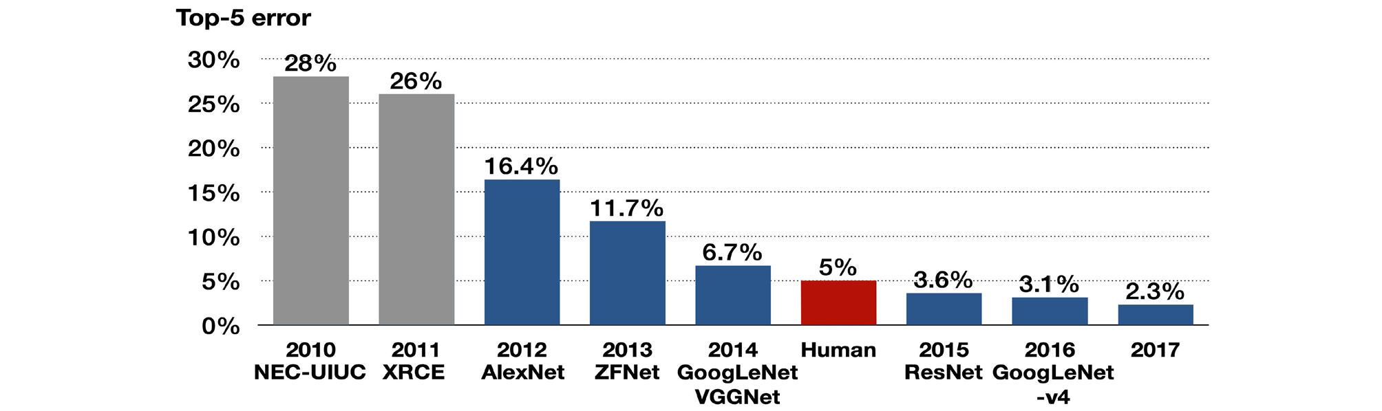
Fig. 2.

Algorithms that won the ImageNet Large Scale Visual Recognition Challenge (ILSVRC) in 2010– 2017. The top-5 error refers to the probability that all top-5 classifications proposed by the algorithm for the image are wrong. The algorithms with blue graph are convolutional neural network. Although VGGNet took second place in 2014, it is widely used in studies as its concise structure. Adapted from “A fully-automated deep learning pipeline for cervical cancer classification” by Alyafeai Z., Ghouti L., Expert Systems with Applications Proceedings of the IEEE 2019;141;112951. Copyright 2019 by Elsevier Ltd.

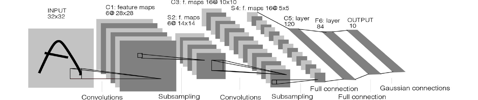
The origin of the CNN is the Neocognitron Model,³ which applied a neurophysiological theory to an artificial neural network based on the principle that only certain neurons in the visual cortex are activated according to the shape of target object.⁴ CNNs largely comprise three layers: convolutional layer, pooling layer, and fully connected layer. The convolutional layer creates a feature map by arranging the outputs of convolution operation at each position of square filter while the filter is sliding over the input data. It has the advantage of preserving horizontal and vertical information among pixels compared to the fully connected neural network, which converts images to one-dimensional vector. The pooling layer downsamples size of the feature map and summarizes important information in the feature map; the classification value is then output through the fully connected layer. For example, LeNet, which was the first CNN that classified hand-written numbers with an error rate of 0.95%, comprises three convolutional layers, three pooling layers, and one fully connected layer (Fig. 3).⁵

Fig. 3.

Architecture of LeNet-5. Reprinted from “Gradient-based learning applied to document recognition” by LeCun Y., Bottou L, Bengio Y. et al., Proceedings of the IEEE 1998;86;2278–2323. Copyright 1998 by IEEE.

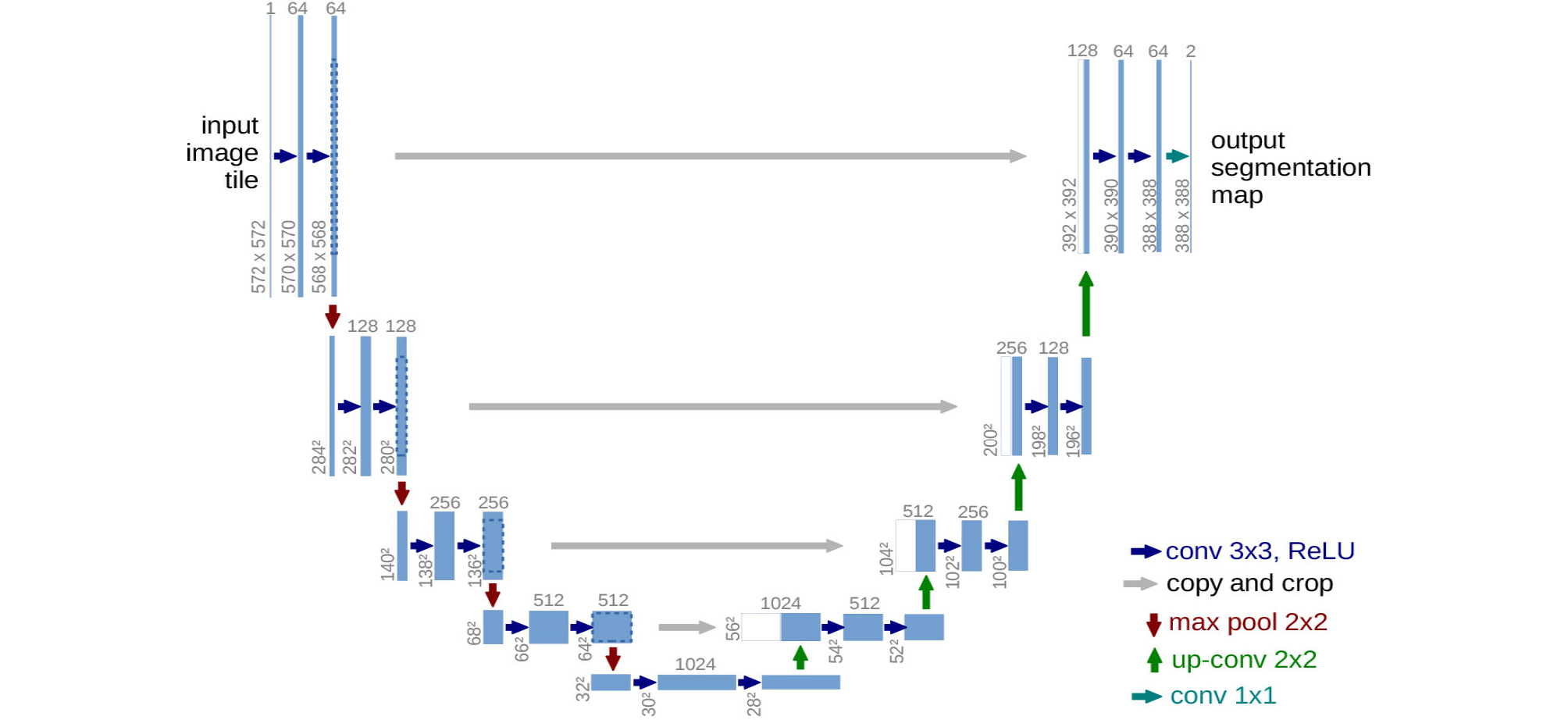
Meanwhile, U-Net, which is used for region segmentation of medical images, does not have a fully connected layer. It comprises an encoder part, which extracts a feature map by convolution and pooling, and a decoder part, which restores the segmented images from the feature map by “up-convolution” (Fig. 4).⁶

Fig. 4.

Architecture of U-net. Reprinted from “U-net: Convolutional networks for biomedical image segmentation” by Ronneberger O., Fischer P., Bottou L, Brox T., Lecture Notes in Computer Science 2015;9351:234-241. Copyright 2015 by Elsevier Ltd.

When detecting multiple objects in a single image, a region-based CNN (R-CNN) is used, which includes a region proposal network for the recognition of objects and their positions (Fig. 5).⁷ The region proposal network suggests anchor boxes of various ratios and sizes for the input image, and those that have a high intersection-over-union (IOU) with the previously trained images are selected.

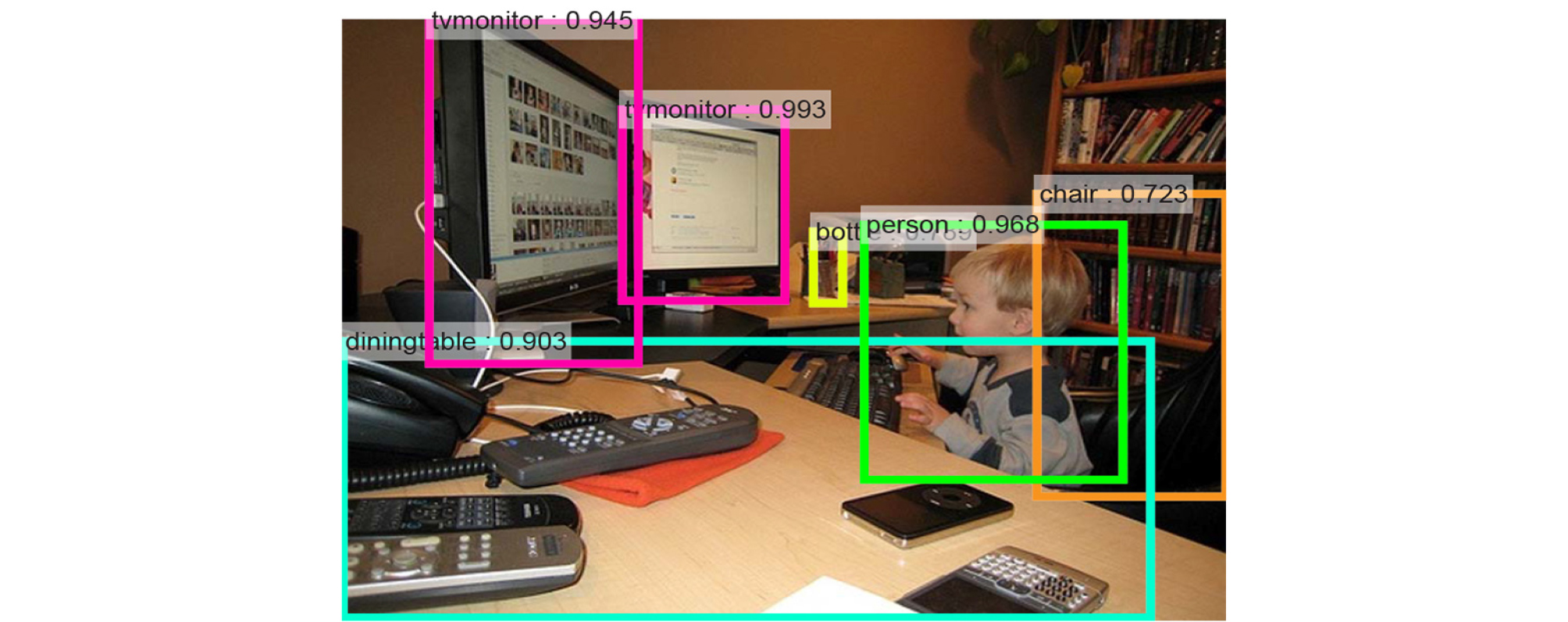
Fig. 5.

Multiple object recognition in region-based convolutional neural network. Reprinted from “Faster R-CNN: Towards Real-Time Object Detection with Region Proposal Networks” by Ren S., He, K., Girshick, R., Sun, J., IEEE Transactions on Pattern Analysis and Machine intelligence 2017;39(6):1137– 1149.

(2) RNNs

RNNs can analyze time-series data that are arranged in chronological sequence such as voice signals. Therefore, they are utilized to predict indices such as stocks, for voice recognition, text translation, adding image captions, and image or music generation. A video of former US president Barack Obama appearing to give a speech has been published, in which the algorithm synthesize lip motion synchronized with his original voice.⁸ This neural network receives the input values from not only the previous layer (X t ) but also the recurrent neurons of the previous time step, transforms, and delivers them to the next layer and recurrent neurons of the next time step, unlike the feed-forward neural network that only delivers signals from the input layer to the output layer (Fig. 6).

Fig. 6.

Structure of recurrent neural network. Right illustrates unfold structure from left to right over time. Reprinted from http://colah.github.io/posts/2015-08-Understanding-LSTMs/

When an RNN—in a pure sense (also referred to as a “vanilla RNN”)—with the above characteristics is configured with deep layers, there are problems such as gradient vanishing/exploding and the longterm dependency. To solve these problems, changes in connections among cells (the units of neural networks) including skip connection or leaky units, long short-term memory cells,⁹ and gated recurrent unit cells¹⁰ using gates inside the cells have been proposed.

(3) GANs

GANs are unsupervised learning algorithms,¹¹ which have a neural network generating an answer inside a neural network (the generator) competes with a neural network that evaluates it (the discriminator). The fake answers proposed by the generator are gradually similar to the ground truth with the aid of the feedback from the discriminator.

2) Output data of deep learning

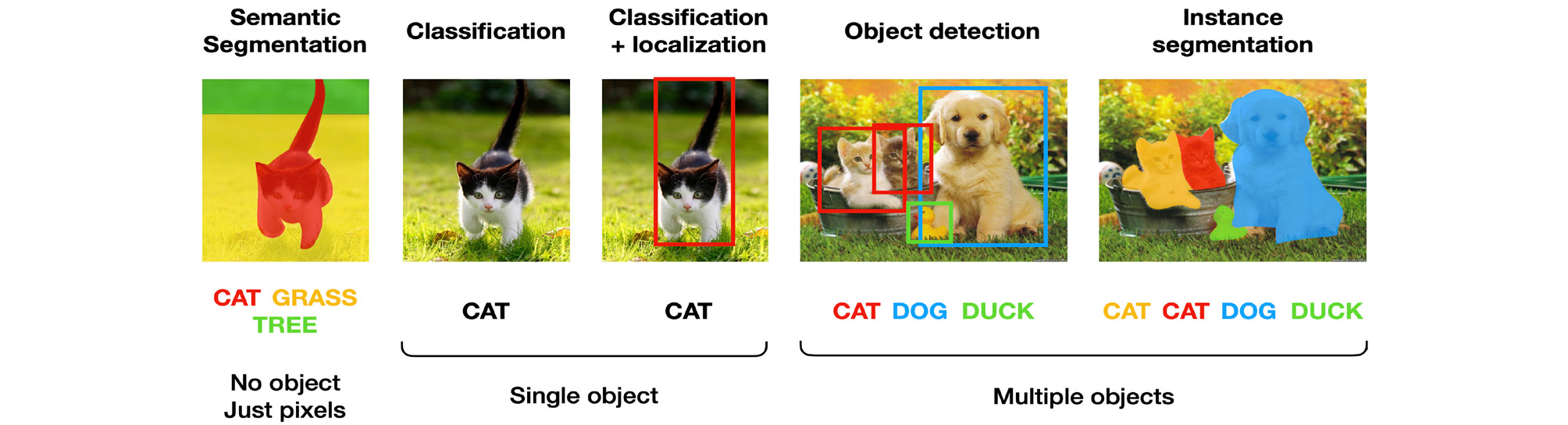
The results of deep learning image analysis can be largely divided into five types as follows (Fig. 7). (1) Classification: The objects in image are classified as the most likely option to be ground truth among predetermined options. One example is LeNet-5, which classified hand-written numbers into 10 types, from 0 to 9. (2) Object localization: This is to indicate the locations of objects in image by bounding boxes. When object localization and classification are performed simultaneously, it is called object detection. (3) Semantic segmentation: This means to segment whole image according to the pixel-based classification without object recognition. (4) Instance segmentation: This recognizes each object and delineates its outline in an image. (5) Image reconstruction: Examples include image quality enhancement by super-resolution or artifact reduction, and class activation maps overlap heat map, which changes the color depending on the contribution of the classification, to the input image. This allows visual confirmation based on which areas of the image are classified using the deep learning algorithm.

Fig. 7.

Computer vision tasks. Adapted from “https://www.slideshare.net/darian_f/introduction-to-theartificial-intelligence-and-computer-vision-revolution.”

3) Performance metrics of deep learning algorithms

The representative performance metrics for classification algorithms are accuracy, precision, recall, F1 score, and the area under the receiver operating characteristic curve (AUC). Other metrics except AUC can be calculated using the confusion matrix illustrating whether the predicted classification matches the ground truth (Fig. 8).

Fig. 8.

Confusion matrix to calculate accuracy (A) and to calculate precision recall, and F1 score (B).

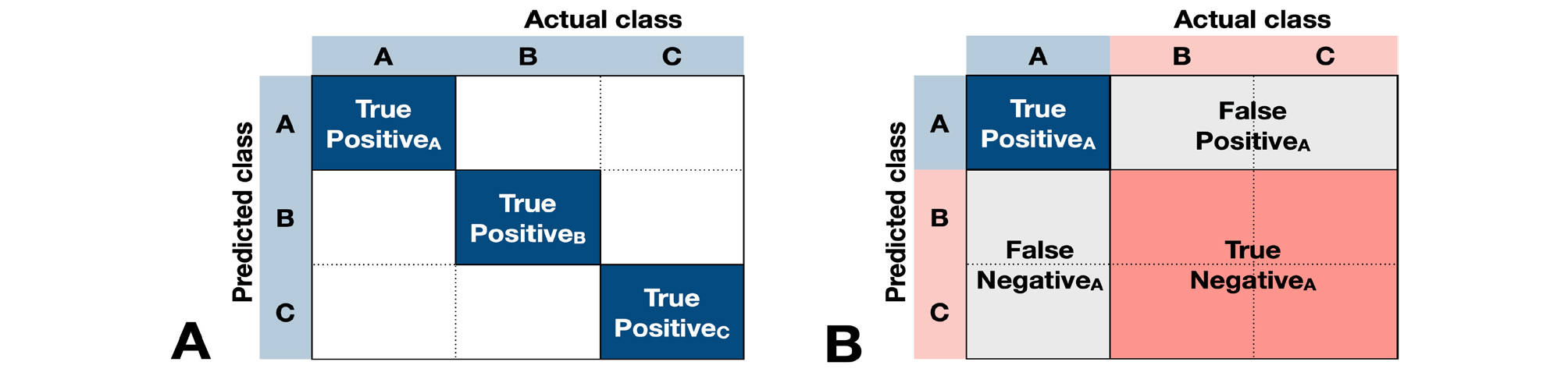
For example, when we evaluate the accuracy of a deep learning model that classifies images into three types, we can calculate the accuracy simply by dividing the number of cases which classify A as A, B as B, or C as C by the total number of cases.

$Accuracy=\frac{T{P}_A+T{P}_b+T{P}_c}{Total}$

(TP=True Positive, FP=False Positive, TN=True Negative, FN=False Negative)

Furthermore, the F₁ score can be calculated by determining the precisions (Precision_A, Precision_B, and Precision_C) and recalls (Recall_A, Recall_B, and Recall_C) for classifying A, B, and C, and calculating the mean precision (Precision_mean) and mean recall (Recall_mean), and then calculating the harmonic mean of these two.

$$\begin{gathered} Precisio{n}_A=\frac{T{P}_A}{T{P}_A+F{P}_A}, \\ Recal{l}_A=\frac{T{P}_A}{T{P}_A+F{N}_A}, \\ {F}_{1}score=\frac{2}{{\displaystyle \frac{1}{Precisio{n}_{mean}}}+{\displaystyle \frac{1}{Recal{l}_{mean}}}}\left(harmonicmean\right) \end{gathered}$$

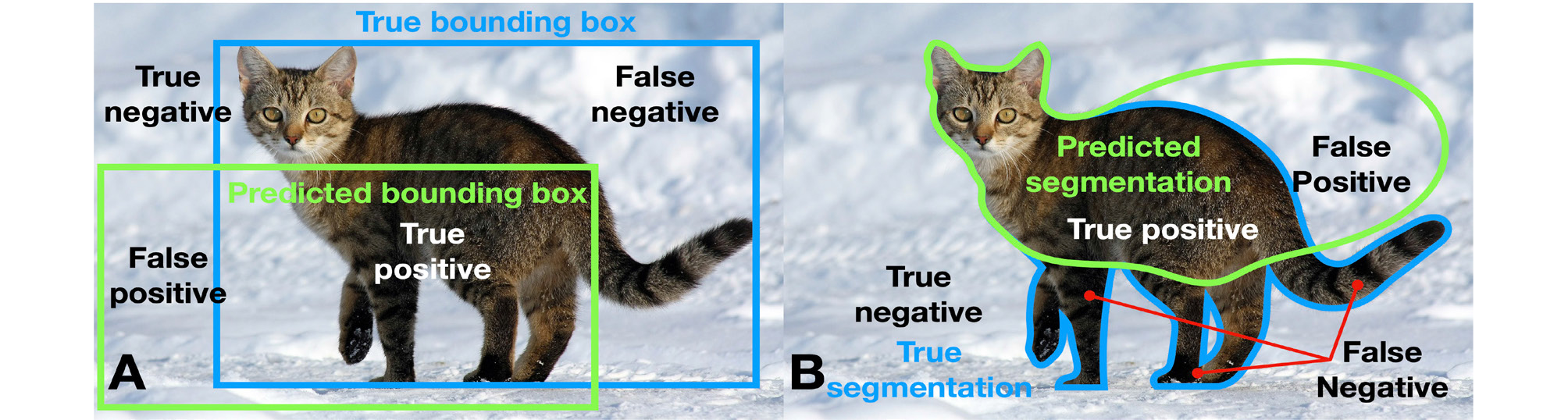
The evaluation indices for object localization and segmentation include the IOU and the dice similarity coefficient, in addition to the above-mentioned indices (Fig. 9). IOU is also called Jaccard index and is calculated by dividing the overlapping area between the ground truth and the predicted areas by the union area. The dice similarity coefficient is calculated by dividing the double of the overlapping area by the sum of each area.

Fig. 9.

Evaluation of object localization (A) and object segmentation (B).

$IOU=\frac{\left|A\cap B\right|}{\left|A\cup B\right|}=\frac{TP}{TP+FP+FN},DSC=\frac{2\left|A\cap B\right|}{\left|A\right|+\left|B\right|}=\frac{2TP}{2TP+FP+FN}$

Ⅲ. Results

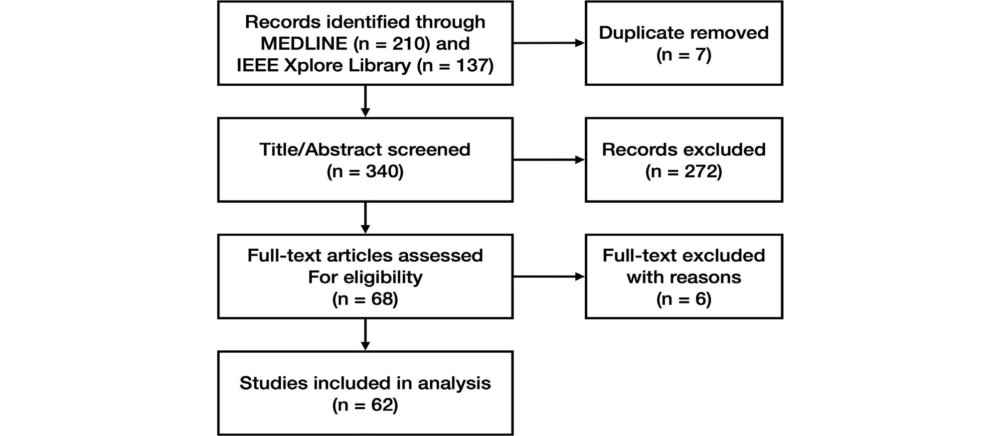
1. Literature Search and Selection of Studies

We found 340 papers by searching MEDLINE and the IEEE Xplore Library, excluding 7 duplicates. After evaluating the titles and abstracts, we excluded 272 papers and evaluated the full texts of 68 papers. A total of 62 papers were included in the study (Fig. 10). The excluded papers and the reasons for their exclusion are outlined in Suppl. 1.

Fig. 10.

Flow chart showing literature search and selection.

2. Data Extraction

The characteristics of the selected studies and the extracted data are listed in Table 2.

Table 2.

Characteristics of included studies

Author Year	Architecture	Input	Output			Performance metrics
1. Detection and segmentation of tooth and oral anatomy
1.1 Tooth localization and numbering
Eun 201674	Sliding window technique with CNN	7,662 backgrounds, 651 single-root teeth, and 484 multi-root teeth images cropped from 500 periapical radiographs	Multiple object localization(tooth)		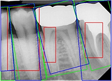	Mean average best overlap=0.714
			Classification (background, single-root tooth, multi-root tooth)			None
Oktay 201775	Sliding window technique with CNN(AlexNet)	100 panoramic radiographs	Classification (anterior, premolar, molar)		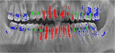	Accuracy(anterior)=0.9247, Accuracy (premolar) =0.9174, Accuracy(molar) =0.9432
Miki 201776	CNN (AlexNet)	Cropped CBCT slices from 52 participants (227×227 pixel)	Classification (central incisor, lateral incisor, canine, 1st premolar, 2nd premolar, 1st molar, 2nd molar)	-		Dataset D (rotation & gamma correction) Accuracy=0.888
Zhang 201814	Cascade network = 3 CNNs(ImageNet pre-trained VGG16) + 1 logic refine module	1,000 periapical radiographs	Multiple object localization(tooth)		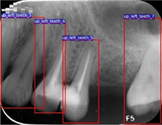	Precision=0.980, Recall=0.983, F1 score=0.981
			Classification (tooth numbering)			Precision=0.958, Recall=0.961, F1 score=0.959
Chen 201912	Faster R-CNN with inception ResNet v2	1,250 periapical radiographs [(300-500)× (300-4 00] pixel)	Multiple object localization(tooth)		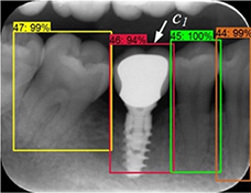	Precision=0.900, Recall=0.985, IOU=0.91
			Classification (tooth numbering)			Precision=0.715, Recall=0.782
Tuzoff 201913	Faster R-CNN with VGG16	1,574 panoramic radiographs	Multiple object localization(tooth)		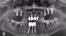	Precision=0.9945, Recall†=0.9941
			Classification (tooth numbering)			Specificity =0.9994, Recall†=0.9800
	Expert		Multiple object localization(tooth)			Precision=0.9998, Recall†=0.9980
			Classification (tooth numbering)			Specificity =0.9997, Recall†=0.9893
Koch 201977	6 modifications of U-Net	1,500 panoramic radiographs	Classification(1-4: 32, teeth with/without restoration and with/without orthodontic appliance, 5: implant, 6: >32 teeth , 7-10: <32 teeth with/without restoration and with/without orthodontic appliance)		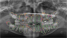	Ensemble of U-Net modification 1 and 4 Accuracy=0.952, Precision=0.933, Recall†=0.944, Specificity=0.961, DSC=0.936
	Mask R-CNN					Accuracy=0.98, Precision=0.94, Recall†=0.84, Specificity=0.99, DSC=0.88
Hiraiwa 201978	CNN(AlexNet)	760 cropped images of mandibular 1st molar from 400 panoramic radiographs CBCT images from 400 participants (ground truth)	Prediction(number of distal root of mandibular 1st molar)		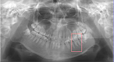	Accuracy=0.874, Recall†=0.773, Specificity=0.971, Precision†=0.963, NPV=0.818, AUC=0.87, Training time =51 minutes, Testing time =9 seconds
	CNN(GoogleNet)					Accuracy=0.853, Recall†=0.742, Specificity=0.959, Precision†=0.947, NPV=0.800, AUC =0.85, Training time =3 hours, Testing time =11 seconds
	Expert radiologist					Accuracy=0.812, Recall†=0.802, Specificity=0.820 Precision†=0.787, NPV=0.834, AUC=0.74
1.2. Tooth segmentation
Jader 201815	Mask R-CNN with ResNet101	1,500 panoramic radiographs	Instance segmentation		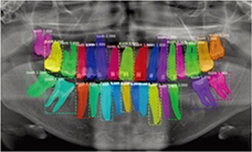	None
			Classification(1-4: 32, teeth with/without restoration and with/without orthodontic appliance, 5: implant, 6: >32 teeth , 7-10 <32 teeth with/without restoration and with/without orthodontic appliance)			Accuracy=0.98, Precision=0.94, Recall=0.84, F1 score=0.88, Specificity=0.99
Vinayahalingam 201979	CNN(U-Net)	81 panoramic radiographs	Instance segmentation (3rd molar)		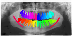	DSC=0.936, IOU=0.881, Recall†=0.947, Specificity=0.999
			Segmentation (mandibular canal)			DSC=0.805, IOU=0.687, Recall†=0.847, Specificity=0.967
De Tobel 201721	CNN(ImageNet pre-trained AlexNet)	20 cropped images of lower left 3rd molar (240×390 pixel) from 20 panoramic radiographs	Classification (modified Demirjian's staging, 0-9)		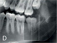	Mean accuracy =0.51, Mean absolute difference =0.6 stages
Merdietio 201916	CNN(AlexNet)	400 panoramic radiographs	Segmentation (lower left 3rd molar)			Accuracy=0.61
			Classification (Modified Demirjian's staging, 0-9)			Accuracy=0.61 Mean absolute difference =0.53 stages Cohen's 𝜅 linear =0.84
Tian 201917	CNN (sparse octree structure, voxel-based)	3D scanned images of 600 dental models	Classification (tooth numbering)		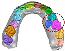	Recall†=0.9800, Specificity=0.9994
			Instance segmentation(tooth)			Accuracy=0.8981
	Expert		Classification (tooth numbering)			Recall†=0.9893, Specificity=0.9997
Xu 201918	CNN	3D scanned mesh images from 1,200 dental models	Instance segmentation (tooth-gingiva, tooth-tooth)		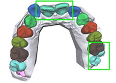	Accuracy(maxilla)=0.9906 Accuracy (mandible) =0.9879
1.3. Bone segmentation
Duong 201920	CNN(U-Net)	50 intraoral ultrasonic images on 8 lower incisors from piglets (128×128 pixel)	Segmentation (alveolar bone)		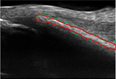	DSC=75.0±12.7%, Recall† =77.8±13.2%, Specificity =99.4±0.8%
Minnema 201919	CNN(MS-D Net)	CBCT from 20 patients	Segmentation(bone)			DSC=0.87±0.06, Mean absolute deviation =0.44 mm
	CNN(U-Net)		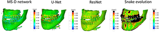			DSC=0.87±0.07, Mean absolute deviation =0.43 mm
	CNN(ResNet)					DSC=0.86±0.05, Mean absolute deviation =0.40 mm
	Snake evolution algorithm					DSC=0.78±0.07, Mean absolute deviation =0.57 mm
2. Image quality enhancement
Du 201822	CNN	Center-cropped images from 5,166 panoramic radiographs (256×256 or 384×384 pixel)	Image reconstruction (compensating blurring from the positioning error)		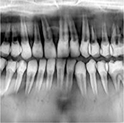	Model 1 Mean standard error=0.339, Mean absolute error=0.749, Maximum absolute error=1.499
Liang 201823	Hanning + filtered back projection	CBCT from 3,872 patients	Image reconstruction (noise and artifact reduction)		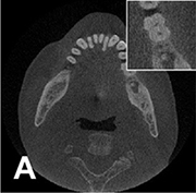	Root mean square error=0.1180, SSI=0.9670
	Non-local mean weighted least square iterative reconstruction		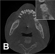			Root mean square error =0.0862, SSI=0.9839
	Network reconstruction		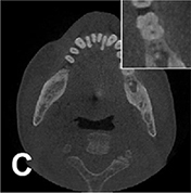			Root mean square error =0.1015, SSI=0.9800
Hu 201924	GAN	Low-dose CBCT images from 44 patients 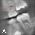(180 180°scanned images, 120 360° scanned images)	Image reconstruction (noise and artifact reduction)		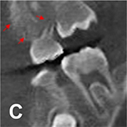	PSNR(360°) =32.657, SSI(360°)=0.925, Noise suppression=5.52±0.25, Artifact correction=6.98±0.35, Detail restoration=5.56±0.31, Comprehensive quality =6.52±0.34, Training time per batch=0.691, Testing time per batch=0.183
	CNN		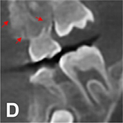			PSNR(360°) =34.402, SSI(360°)=0.934, Noise suppression =8.95±0.36, Artifact correction =7.20±0.23, Detail restoration =5.35±0.28, Comprehensive quality =7.54±0.32, Training time per batch=0.726, Testing time per batch =0.183
	m-WGAN	Normal dose CBCT images (ground truth)	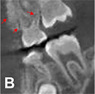		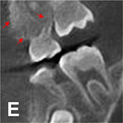	PSNR(360°) =33.824, SSI(360°)=0.975, Noise suppression =8.20±0.35, Artifact correction =7.46±0.27, Detail restoration=8.98±0.20, Comprehensive quality =8.25±0.21, Training time per batch=0.798, Testing time per batch =0.184
Hegazy 201925	CNN(U-Net)	1,000 projection images (0-180°) from 5 patients who had different kinds of metal implants and dental fillings at different tooth positions	Segmentation (metal)		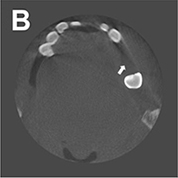	Mean IOU=0.94 Mean DSC=0.96
			Image reconstruction (metal artifact reduction)			Mean relative error =94.25% Mean normalized absolute difference =93.25% Mean sum of square difference =91.83%
	Conventional segmentation method	Original CBCT images	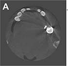Segmentation (metal)		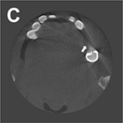	Mean IOU=0.75 Mean DSC=0.86
			Image reconstruction (metal artifact reduction)			Mean relative error =91.71% Mean normalized absolute difference =95.06% Mean sum of square difference =93.64%
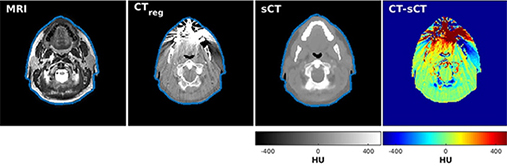
Dinkla 201926	CNN(U-Net)	3D patch (48×48×48 voxel) from 34 head and neck T2-weighted MRI CT(ground truth)	Image reconstruction (synthetic computed tomography)			Comparing synthetic CT and conventional CT, Mean DSC=0.98±0.01, Mean absolute error =75±9 HU Mean error =9±11 HU, Mean voxel-wise dose differences =-0.07±0.22%, Mean gamma pass rate=95.6±2.9%. Mean dose difference=0.0±0.6%(body volume), -0.36±2.3% (high-dose volume)
Hatvani 201927	CBCT(original)	CBCT of 13 teeth (linewidth resolution=500μm, voxel size =80×80×80μm3), Micro-CT of 13 teeth (linewidth resolution=50μm, voxel size=40×40×40μm3) (ground truth)	Image reconstruction (super-resolution)	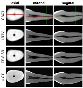		DSC=0.88 Mean of difference - Feret=176, Mean of difference - Area=0.1139
	LRTV					DSC=0.89, Time=6988 (maxillary anterior teeth), 9059(mandibular premolar), 10301 seconds (mandibular molar), Mean of difference - Feret=113, Mean of difference - Area =0.1395
	TF-SISR					DSC=0.90, Time=71 (maxillary anterior teeth), 92(mandibular premolar), 104 seconds (mandibular molar), Mean of difference - Feret =95, Mean of difference - Area =0.0987
Hatvani 201928	CBCT(original)	5,680 CBCT slices of 13 teeth 5,680 micro-CT slices of 13 teeth (ground truth)	Image reconstruction (super-resolution)	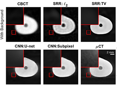		DSC=0.8891, Difference of the endodontic volumes (CBCT- μCT) =12.39%
	SRR:l2					DSC=0.8852 Difference of the endodontic volumes (SRR:l2- μCT) =12.25%
	SRR:TV					DSC=0.8913 Difference of the endodontic volumes (SRR:l2- μCT) =12.40%
	CNN (U-Net)					DSC=0.8998 Difference of the endodontic volumes (U-net- μCT) =10.12%
	CNN (Subpixel network)					DSC=0.9101 Difference of the endodontic volumes (Subpixel network-μCT) =6.07%
3. Disease detection
3.1. Detection of dental caries
Kumar 201829	CNN(U-Net)	>6,000 bitewing radiographs	Instance segmentation (dental caries)		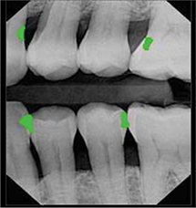	Recall=0.70, Precision=0.53, F1 score=0.603
	CNN(U-Net) + incremental example mining					Recall=0.73, Precision=0.53, F1 score=0.614
	CNN (U-Net) + hard example mining					Recall=0.69, Precision=0.46, F1 score=0.552
Lee 201930	CNN (ImageNet pre-trained GoogleNet Inception v3)	3,000 periapical radiographs	Classification (caries, non-caries)	-		Accuracy=82.0, Recall†=81.0, Specificity=83.0, Precision†=82.7, NPV=81.4 in premolar and molar area
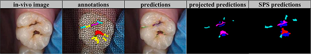
Casalegno 201931	CNN (encoding path of U-Net replaced with the ImageNet Pre-trained VGG16)	217 near-infrared transillumination images (256×320 pixel)	Semantic segmentation (background, enamel, dentin, proximal caries, occlusal caries			Mean IOU=0.727, IOU(proximal caries)=0.495, IOU(occlusal caries)=0.490, AUC(proximal caries)=0.856, AUC(occlusal caries)=0.836
Moutselos 201932	Mask R-CNN with ResNet101	79 clinical photos of occlusal surface	Classification in superpixel level (international caries detection and assessment system 0: sound tooth surface, 1: first visual change in enamel, 2: distinct visual change in enamel, 3: localized enamel breakdown, 4: underlying dark shadow from dentin, 5: distinct cavity with visible dentine, 6: extensive distinct cavity with visible dentin)			F1 score(mc) =0.596, F1 score(cpc) =0.625, F1 score(wc) =0.684 3 indexes for the reduction back to superpixels (mc: most common, cpc: centroid pixel class, wc: worst class)
			Classification in whole image level			F1 score(mc) =0.889, F1 score (cpc) =0.778, F1 score (wc) =0.667
Liu 201934	Mask R-CNN with ResNet	12,600 clinical photos(1 mega pixel)	Multiple object localization, classification (dental caries, dental fluorosis, periodontitis crack tooth, dental plaque, dental calculus, tooth loss)		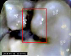	Accuracy: 0.875 (tooth fluorosis)-1 (tooth loss), increase of the number of treated patients by 18.4%, mean diagnosis time reduces by 37.5% for each patient
3.2. Detection of dental plaque and periodontal disease
Yauney 201780	CNN (truncated version of VGG16)	47(CD database) and 49(RD database) pairs of white light mode and plaque mode intraoral photo (512×384 pixel)	Semantic segmentation (plaque, non-plaque)			Accuracy=0.8718, AUC=0.8720
Bezruk 201735	CNN	Malondialdehyde concentration, Gluthatione concentration, Sulcus bleeding index	Classification (normal, gingivitis)	-		Precision=0.80, Recall=0.78, F1 score=0.78
Aberin 201836	CNN(AlexNet)	1,000 grayscale images with 600 magnification (227×227 pixel)	Classification (healthy, unhealthy)		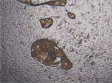	Accuracy=0.76, Mean square error =0.05, Precision=0.68, Recall=0.98
Joo 201937	CNN	1,843 clinical photos of periodontal tissue	Classification (healthy periodontal status, mild periodontitis, severe periodontitis, not periodontal image)	-		Accuracy(healthy)=0.83, Accuracy(mild periodontitis) =0.74, Accuracy(severe periodontitis) =0.70, Accuracy(not periodontal image)=0.94
Krois 201938	CNN	2,001 cropped panoramic radiographs	Classification (<20% bone loss, ≥20% bone loss)	-		Accuracy=0.81, Precision†=0.76, Recall†=0.81, Specificity=0.81, NPV=0.85, AUC=0.89, F1 score=0.78
	Dentist					Accuracy=0.76, Precision†=0.68, Recall†=0.92, Specificity=0.63, NPV=0.90, AUC=0.77, F1 score=0.78
3.3. Detection of periapical diseases
Prajapati 201733	CNN (2012 ImageNet pre-trained VGG16)	251 periapical radiographs (500×748 pixel)	Classification (dental caries, periapical infection, periodontitis)	-		Accuracy=0.8846
Ekert 201944	CNN	1,331 cropped panoramic radiographs of 85 patients (64×64 pixel)	Classification (no attachment loss, widened periodontal ligament, clearly detectable lesion)			Recall† =0.74±0.19, Specificity =0.94±0.04 Precision† =0.67±0.14, NPV=0.95±0.04 AUC=0.95±0.02 In all teeth, majority(6) reference test condition
Yang 201882	CNN(GoogLeNet Inception v3)	196 pairs of periapical radiograph before and after the treatments (96×192 pixel)	Classification (getting better, getting worse, have no explicit change)			Precision=0.537, Recall=0.490, F1 score=0.517
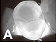
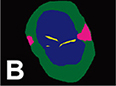
3.4. Detection of (pre)cancerous lesion
Uthoff 200839	CNN	170 pairs of Autofluorescence image and white light image	Classification (cancerous and pre-cancerous lesion, not suspicious)		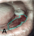	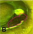Precision† =0.8767, Recall† =0.8500, Specificity =0.8875, NPV=0.8549, AUC=0.908;
	Remote specialist					Precision† =0.9494, Recall† =0.9259, Specificity =0.8667, NPV=0.8125
Aubreville 201740	CNN +Probability fusion	165,774 patches extracted from 7,894 grayscale confocal laser endomicroscopy video frames of the inner lower labium, the upper alveolar ridge, the hard palate (80×80 pixel)	Classification (normal, cancerous)		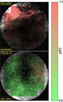	Accuracy=0.883, Recall†=0.866, Specificity=0.900, AUC=0.955
Forslid 201741	CNN (VGG16, ResNet18)	Oral dataset 1 (15 microscopic cell images taken at ×20 magnification)	Classification (healthy, tumor)	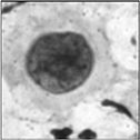VGG16		ResNet18
				Accuracy=80.66±3.00, Precision=75.04±7.68, Recall=80.68±3.05, F1 score=77.68±5.28		Accuracy =78.34±2.37, Precision =72.48±4.46, Recall =79.00±3.37, F1 score 75.51±3.17
		Oral dataset 2 (15 microscopic cell images taken at ×20 magnification)		Accuracy=80.83±2.55, Precision=82.41±2.55, Recall=79.79±3.75, F1 score=81.07±3.17		Accuracy =82.39±2.05, Precision =82.45±2.38, Rcall =82.58±1.92, F1 score 82.51±2.15
		CerviSCAN dataset (12,043 microscopic cell images taken at ×40 magnification)		Accuracy=84.20±0.86, Precision=84.35±0.97, Recall=84.20±0.86, F1 score=84.28±0.91		Accuracy =84.45±0.46, Precision =84.64±0.38, Rcall =84.45±0.47, F1 score 84.28±0.91
		Herlev dataset (917 microscopic cell images)		Accuracy=86.56±3.18, Precision=85.94±6.98, Recall=79.04±3.81, F1 score=82.16±3.85		Accuracy =86.45±3.81, Precision =82.45±5.11, Recall =84.45±2.16, F1 score 83.36±3.65
Das 201842	CNN	1,000,000 patches from 80 microscopic images taken at ×50 magnification (2,048×1,536 pixel)	Semantic segmentation (keratin, epithelial, subepithelial, 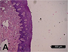background)		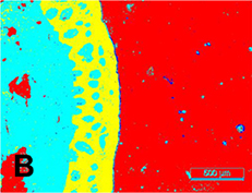	Accuracy (epithelial) =0.984, Recall† (epithelial) =0.978, IOU(epithelial) =0.906, DSC(epithelial) =0.950, Accuracy(keratin) =0.981, IOU(keratin) =0.780, DSC(keratin) =0.752
			Multiple object localization (keratin pearl)			Accuracy=0.969
Jeyaraj 201943	SVM	1,300 image patches from 3 databases (BioGPS data portal=100, TCIA Archive=500, GDC Dataset=700)	Classification (normal, benign tumor, cancerous malignant)	-		Accuracy=0.82, Specificity=0.86, Recall†=0.76, AUC=0.725
	DBN					Accuracy=0.85, Specificity=0.89, Recall†=0.82, AUC=0.85
	CNN					Accuracy=0.91, Specificity=0.94, Recall†=0.91, AUC=0.965
Song 201983	Central attention residual network in CNN	48 tissue microarray core images (3,300×3,300 pixel)	Classification (tumor, stroma)		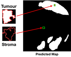	F1 score(RGB) =86.31% DSC(RGB) =82.16%
3.5. Detection of other disease
Murata 201945	CNN(AlexNet)	800 cropped panoramic radiographs of maxillary sinus (200×200 pixel)	Classification (healthy, inflamed)			Accuracy=0.875, Recall†=0.867, Specificity=0.883, Precision†=0.881, NPV=0.869, AUC=0.875
	Radiologist					Accuracy=0.896, Recall†=0.900, Specificity=0.892, Precision†=0.893, NPV=0.899, AUC=0.896
	Dental residents					Accuracy=0.767, Recall†=0.783, Specificity=0.750, Precision†=0.758, NPV=0.776, AUC=0.767
De Dumast 201846	NN	293 condyle images from reconstructed CBCT	Classification(close to normal[control], close to normal [osteoarthritis], degeneration 1,2,3,4-5)			In confusion matrix, Accuracy=0.441, Accuracy (including adjacent 1 cell around true positive cell)=0.912
Kise 201947	CNN(AlexNet)	500 cropped CT images of parotid gland in 25 patients	Classification (normal, Sjögren syndrome)		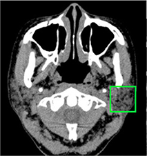	Accuracy=0.96, Recall†=1, Specificity=0.92, AUC=0.960
	Experienced radiologist					Accuracy=0.983, Recall†=0.993, Specificity=0.779, AUC=0.996
	Inexperienced radiologist					Accuracy=0.835, Recall†=0.779, Specificity=0.892, AUC=0.997
Chu 201848	Octuplet Siamese network with 2-stage fine tuning	864 cropped panoramic radiographs (50×50 pixel)	Classification (normal, osteoporosis)			Accuracy=0.898
Kats 201949	Faster R-CNN (ResNet101)	65 panoramic radiographs	Multiple object localization (atherosclerotic carotid plaques)		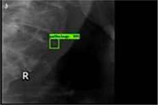	Accuracy=0.83, Recall†=0.75 Specificity=0.80, AUC=0.83
4. Evaluation of facial esthetics, detection of cephalometric landmarks
Murata 201750	CNN (ImageNet pre-trained VGG19) + LSTM	352 patients' images (304×224 pixel) 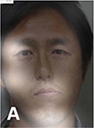Mouth/left	Classification (mouth, jaw, face) 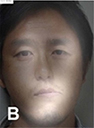Jaw/left	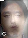Face/remarkably distortion		Accuracy=0.648
	Multiple CNNs					Accuracy=0.630
Patcas 201951	CNN (Internet Movie database- Wikipedia pre-trained, APPA-REAL and Chicago Face Dataset fine-tuned VGG16)	2,164 facial images of pre-/post-operation (Le Fort I osteotomy, sagittal split ramus osteotomy of the mandible, chin osteotomy, other osteotomies, 600 dpi)	Prediction apparent age, facial attractiveness (0-100, 0: extremely unattractive, 100: extremely attractive)			Mean difference between apparent age and actual age (pre-operation) =1.75 year Mean difference between apparent age and actual age (post-operation) =0.82 years Facial attractiveness was increased at 74.7% of patients
Leonardi 201052	Cellular NN (unsupervised learning)	40 lateral cephalometric radiographs, 22 landmarks	Image reconstruction (emboss enhancement)		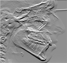	Euclidean distance mean errors: higher for the embossed images than for the unfiltered radiographs Accuracy of the cephalometric landmark detection improved on the embossed radiograph but only for a few points, without statistical significance
Qian 201953	Faster R-CNN with VOC 2012 pre-trained ResNet50)	400 lateral cephalometric radiographs	Multiple object localization (19 landmarks)		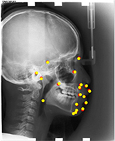	Accuracy(test 1) =0.825, Accuracy(test 2) =0.724 Landmark can be classified as a 'accurate' on only if the distance between a detected landmark and its ground truth is less than 2 mm.
Torosdagli 201954	CNN (U-Net, deep geodesic learning), LSTM	25,600 slices from 50 3D reconstruced CBCT	Segmentation (mandible)		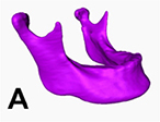	DSC=0.9386, Hausdorff distance=5.47
			Multiple object localization (landmarks on mandible)		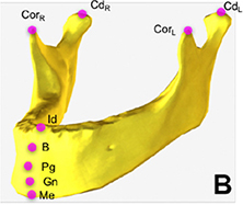	Mean error(mm): coronoid process(left)=0, coronoid process(right) =0.45, condyle(left) =0.33, condyle(right) =0.07, menton=0.03, gnathion=0.49, pogonion=1.54, B-point=0.33, infradentale=0.52
5. Fabrication of prosthesis
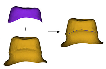
Shen 201984	CNN(U-Net)	77 single crown models	Prediction (deformation, translation, scaling down, rotation)			F1 score (deformation) =0.9614, F1 score (scaling down) =0.9408, F1 score (translation) =0.9386, F1 score (rotation) =0.9387
			Image reconstruction (compensating deformation, translation, scaling down, rotation)			F1 score (deformation) =0.9699, F1 score (scaling down) =0.9488, F1 score (translation) =0.9517, F1 score (rotation) =0.9417
Shen 201955	CNN(U-Net)	28,433 slices from 71 3D single crown models (256×256 pixel)	Prediction (deformation, scaling down, rotation)			Recall (deformation) =1.000, Recall (scaling down) =0.984, Recall (rotation) =0.982, Precision (deformation) =1.00 0, Precision (scaling down) =0.993, Precision (rotation) =0.978, F1 score (deformation) =1.000, F1 score (scaling down) =0.989, F1 score (rotation) =0.980
			Image reconstruction (compensating deformation, scaling down, rotation)			Recall (deformation) =1.000, Recall (scaling down) =0.993, Recall (rotation) =0.983, Precision (deformation) =1.000, Precision (scalin down) =0.991, Precision (rotation) =0.980, F1 score (deformation) =1.000, F1 score (scaling down) =0.992, F1 score (rotation) =0.982
Yamaguchi 201956	CNN	8,640 3D scan images of study model (100×100 pixel)	Classification (trouble-free, debonding)			Accuracy=0.985, Precision=0.970, Recall=1, F1 score=0.985, AUC=0.098
Zhang 201957	CNN (sparse octree structure, voxel-based)	From 380 preparation models: dataset A: no rotation	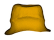Segmentation(preparation line)			Accuracy=0.9062, Recall†=0.9318, Specificity=0.9458
		dataset B: 60°×5 rotations				Accuracy=0.9558, Recall†=0.9590, Specificity=0.9521
		dataset C: 30°×12 rotations				Accuracy=0.9743, Recall†=0.9759, Specificity=0.9732
Zhao 201958	Convolutional auto-encoder	39,424 models augmented by rotating 77 dental crown models	Prediction(nonlinear deformation)			F1 score (nonlinear deformation, resolution 64×64×64) =0.9684
			Image reconstruction (compensation)			F1 score (nonlinear deformation, resolution 64×64×64) =0.9755 F1 score before compensation (0.7782) was increased after compensation (0.9530)
6. Others
MiloŠević 201959	CNN(ImageNet pre-trained VGG16)	4,000 panoramic radiographs(female= 58.8%, male=41.2%)	Classification (female, male)			Accuracy=96.87±0.96% (filter=256, unit=128, without attention mechanism)
Ilić 201960	CNN(Pre-trained VGG16)	4,155 panoramic radiographs (512×512 pixel)	Classification (female, male)			Accuracy=94.3% (over 80 years=50%), Testing time =0.018 seconds
Alarifi 201885	Radial basis NN	Patient self-behavior, health conditions, attitude information	Prediction (implant success)			Recall†=0.8478, Specificity=0.8678
	General regression NN					Recall†=0.9216, Specificity=0.9351
	Associative NN					Recall†=0.9417, Specificity=0.9482
	Memetic search optimization along with genetic scale RNN					Recall†=0.9763, Specificity=0.9828
Ali 201961	R-CNN(SSD-Mo bileNet)	631 instrument images or video frames (16:9 ratio, 0.5 or 0.67 megapixel)	Multiple object localization, classification (dental instruments)		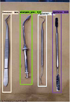	Accuracy=0.87, Precision=0.99, Recall=1, Specificity=0.99
Luo 201962	k-nearest neighbor	3D motion signals caused by the hand movement using wearable devices in 10 participants	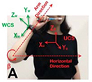Classification (1-15)			Accuracy=0.472
	Support vector machine					Accuracy=0.391
	Decision tree					Accuracy=0.394
	RNN-based LSTM					Accuracy=0.973

3D: three-dimensional; AUC: area under curve; CAD/CAM: computer-aided design/computer-aided manufacturing; CBCT: cone-beam computed tomography; CNN: convolutional neural network; CT: computed tomography; DSC: dice similarity coefficient; GAN: generative adversarial network; HU: Hounsfield unit; ICDAS: international caries detection and assessment system; IOU: intersection-over-union; LSTM: long short-term memory models; LRTV: low-rank and total variation regularizations; m-WGAN: modified-Wasserstein generative adversarial network; NN: neural network; NPV: negative predictive value; PSNR: peak signal-to-noise ratio; R-CNN: region-based convolutional neural network; SSI: structure similarity index; SRR: super-resolution method; TF-SISR: tensor factorization with 3D single image super-resolution.

^*: refers to the data unanimously classified by 6 specialists

^†: sensitivity and positive predictive value were replaced by recall and precision, respectively.

1) Detection of teeth and adjacent anatomical structures

The selected studies in this category can be subdivided into three groups: tooth detection, tooth numbering, tooth segmentation, and bone segmentation. For tooth detection and tooth numbering, panoramic radiographs and cone-beam computed tomography (CBCT) images were used. For multiple object localization of teeth, the precision was reported to be in the range 0.900¹² –0.995¹³ and the recall in the range 0.983¹⁴ –0.994¹³ . The precision of tooth numbering was reported to be in the range 0.715¹² – 0.958¹⁴ and the recall in the range 0.782¹² –0.980¹³.

Tooth segmentation has been attempted for teeth in panoramic radiographs¹⁵ , third molars¹⁶ , and dental model¹⁷, ¹⁸. Algorithms for segmenting bone appearances from CBCT¹⁹ and oral ultrasound images²⁰ have been also proposed. Two studies that classified the developmental stages of third molars reported accuracies of 0.51²¹ and 0.61¹⁶1.

2) Image quality enhancement

For image quality enhancement, studies on the reduction of blur, noise, and metal artifacts as well as on the super-resolution have been conducted. Du et al. corrected blurs in the center of images using an algorithm trained using 5,166 panoramic radiographs taken at positions ±20 mm from the ideal position and the misalignment length (mm), and they reported a maximum absolute error below 1.5 mm.²² Liang et al. reconstructed computed tomography (CT) images using three algorithms and reported improved root mean squared error and structure similarity index compared with the values measured in original CT images.²³ Hu compared a GAN, CNN, and modified GAN using Wasserstein distance and reported that the latter was most effective in the noise reduction from CBCT images.²⁴ Hegazy reported improved the relative error by 5.7%, and the standardized absolute difference by 8.2% using modified U-net algorithm compared to the conventional method.²⁵ Dinkla et al. introduced a U-net-based algorithm that synthesizes CT images with no metal artifacts from T2-weighted magnetic resonance imaging (MRI).²⁶ Hatvani et al. reported a dice similarity index of 0.90 and a mean difference of 9.87% comparing crosssectional area of root canal system of CBCT applied tensor factorization super-resolution algorithm with that of micro CT.²⁷27 They also attempted super-resolution using a subpixel network, reporting a dice similarity index of 0.91 and a mean difference root volume of 6.07% compared with micro CT.²⁸

3) Disease detection

Target diseases include tooth caries,²⁹, ³⁰, ³¹, ³², ³³, ³⁴ periodontal disease,³⁴, ³⁵, ³⁶, ³⁷, ³⁸ precancerous lesions,³⁹, ⁴⁰⁴¹, ⁴², ⁴³ periapical diseases,³³, ⁴⁴ dental fluorosis,³⁴ maxillary sinusitis,⁴⁵ osteoarthritis,⁴⁶ Sjögren ' s syndrome,⁴⁷ and osteoporosis.⁴⁸48 An algorithm for detecting atherosclerotic carotid plaque in panoramic radiographs has been suggested.⁴⁹

4) Evaluation of facial esthetics and localization of cephalometric landmarks

Algorithms for evaluating various images such as facial photographs, lateral cephalometric radiographs, and CBCT images have been proposed. Murata et al. developed an algorithm for classifying the asymmetry and/or discrepancy of crow’s feet, nose, lips, and chin from input frontal face image, and reported an mean accuracy of 64.8%.⁵⁰ Patcas et al. trained CNN-based algorithm to estimate apparent age and facial attractiveness score (0–100 points) using various facial image datasets, and they reported the increased facial attractiveness score (mean difference = 1.22, 95% confidence interval: 0.81, 1.63) and decreased apparent age (mean difference = –0.93, 95% confidence interval: –1.50, –0.36) after orthognathic surgery.⁵¹ Leonardi synthesized embossed images from lateral cephalometric radiograph for enhanced visibility but reported insignificant improvement of reading accuracy.⁵² Qian et al. proposed faster R-CNN method for cephalometric landmark detection. After trained with 150 photographs of 19 types of cephalometric landmarks that were manually localized by expert orthodontist, the method localized landmarks within 2 mm of the landmark located by the orthodontist at 72.4–82.5%.⁵³53 The cephalometric landmarks on the mandible (menton, gnathion, pogonion, B-point, infradentale, coronoid process, condyle head) were localized after segmenting the mandible on the 3D reconstructed CBCT, and an mean error was reported to less than 1 mm except for pogonion.⁵⁴

5) Fabrication of prosthesis

Shen et al. proposed algorithm for predicting and compensating for errors in the cross section of single crown additively manufactured using the 3D printer, and they reported improved F1 scores (translation: 0.6894 → 0.9995, scaling down: 0.7188 → 0.9893, rotation: 0.8906 → 0.9671).⁵⁵55 Yamaguchi developed an algorithm that evaluates the scan data of an abutment preparation model and classified models with a high possibility of debonding and a low possibility (trouble-free), and they reported an accuracy of 98.5%.⁵⁶ In addition, an algorithm that predicts the crown margin in a 3D-scanned abutment preparation model⁵⁷ and an algorithm for predicting the nonlinear deformation of 3D printed crowns from the scan data of an abutment preparation model have been suggested.⁵⁸

6) Others

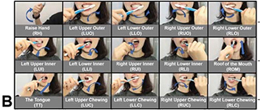
Milosevic and Ilic designed an algorithm for determining sex from panoramic radiographs and reported accuracies of 96.87±0.96%⁵⁹ and 94.3%,⁶⁰ respectively. Ali et al. reported on an algorithm for localizing and classifying dental instruments in image.⁶¹ Luo et al. collected 3D motion signals in daily life using wearable devices and tested four algorithms classifying tooth brushing time and 15 tooth brushing motions. In terms of classifying tooth brushing motions, they reported an mean classification accuracy of 97.3% using the RNN-based algorithm.⁶²

Ⅳ. Discussion

1. Principle of Machine Learning

The basic approach of machine learning is to set a loss function for the difference between the predicted value (ŷ) and the groud truth (y) and determine the global minimum of the loss function based on the fact that accuracy improves as the loss function decreases (Fig. 11).⁶³ One representative example is the least squares method, which squares the differences between each predicted value and the ground truth and minimizes the sum of these differences. The loss function is the mean of the squared differences between the predicted values and the ground truth.

$lossfunction=\frac{1}{m}\sum _{i=1}^m{(y_i-{\hat{y}}_i)}^2$

A basic algorithm for determining the global minimum of the loss function is gradient descent. A smaller input value (χ) is substituted if the gradient of the loss function is positive, and a larger input value is substituted if the gradient is negative, thus converging to the minimum.

Fig. 11.

Schematic diagram showing the training process of machine learning. Adapted from “Deep Learning mit Python und Keras: Das Praxis-Handbuch vom Entwickler der Keras-Bibliothek” by Chollet F., Copyright 2018 by MITP-Verlags GmbH & Co. KG.

2. Development of Deep Learning

Deep learning is a field of machine learning (Fig. 12) and refers to deep artificial neural networks with two or more hidden layers besides the output layer. An artificial neural network is an interconnected group of artificial neurons that perform computations by imitating the brain structure. It started with a simple neural network model with propositional logic,⁶⁴ and artificial neurons called perceptrons⁶⁵ were introduced. However, the exclusive OR operation could not be performed with a single-layer perceptron,⁶⁶ and this problem was solved by developing the backpropagation algorithm for training the multi-layer perceptron.⁶⁷, ⁶⁸ Current deep learning has been improved in performance through the development of a new activation function⁶⁹ to solve the problem of vanishing gradient, while passing through the deep layer of the neural network, optimization of the weighted initialization,⁷⁰, ⁷¹, ⁷² and dropout² for preventing overfitting.

Fig. 12.

Diagram showing the relationship between artificial intelligence, machine learning, and deep learning. Adapted from “Deep Learning mit Python und Keras: Das Praxis-Handbuch vom Entwickler der Keras-Bibliothek” by Chollet F., Copyrights 2018 by MITP-Verlags GmbH & Co. KG.

3. Characteristics and Applicability of the Selected Studies

For application of deep learning to dentistry, an algorithm for detecting multiple objects is required due to the nature of the dental anatomy that multiple teeth are distributed in a single image. For object localization, the sliding window technique was used in early research, which moves the windows of various ratios and sizes in the image in small increments. Later, the object localization became faster with the introduction of the region proposal network embedded in the neural network. Studies on teeth classification performance show slightly different results. To maintain high accuracy even in complex situations such as prosthesis, tooth defect, or mixed dentition, data in various situations need to be trained sufficiently.

If automatic tooth numbering algorithm is combined with classification algorithms for tooth caries, periodontal disease, and root apex disease, it can instantly provide useful clinical information by detecting abnormalities of each tooth. This can be highly beneficial in forensic dentistry as well. Although sex determination using panoramic radiographs shows lower accuracy (94.3%⁶⁰ , 96.87%⁵⁹ ) than using the total skeleton (100%); however, it has the additional advantages that people with partial bones can be analyzed and their dental records can be compared. Analyzing the development stage of third molars can be one of age estimation methods with analyzing hand-wrist radiograph or cervical vertebral maturation in panoramic radiograph.

Studies related to image quality enhancement of dental images mainly have been conducted for CBCT, and development in three directions is anticipated. First, removal of noise due to the scattering of low-energy X-rays, which is the problem of low-dose CT, could increase the number of allowable shots while lowering the radiation exposure of patients, while also maintaining the image quality similar to that of normal dose CT. Second, reducing metal artifacts in the images could be considerably helpful for reading the CT images of patients who have several implants or metal fixed prostheses. For extreme example, Dinkla et al. proposed CNN-based method that synthesizes CT images similar to the existing CT from T2-weighted MRI with no radiation exposure and metal artifacts. Third, high-resolution images can be obtained by applying a super-resolution algorithm to conventional CBCT images. The algorithm was trained by micro CT, which is used experimentally due to its very high exposure in spite of high resolution of µm unit. The super-resolution imaging of CBCT showed similar errors of root canal volume and length to those of micro CT. This is expected to provide great assistance to the diagnosis of teeth with complex root canal systems.

In selected studies, detecting various diseases and risk factors in field of dentistry has been attempted using deep learning, such as dental plaque, dental caries, periodontal disease, and periapical disease, as well as the diseases of adjacent anatomical structures observed in dental images such as the maxillary sinusitis, osteoarthritis of the temporomandibular joint, Sjögren syndrome of the parotid gland, and osteoporosis. Kats et al. reported 83% accuracy when detecting atherosclerotic carotid plaques in panoramic radiographs using an R-CNN.⁴⁹ This algorithm is expected to help diagnose and treat ischemic brain disease because the plaque is known to be significantly associated with strokes.⁷³

When deep learning was applied to the orthodontics, the automatic detection of cephalometric landmarks from radiographs, or facial asymmetry from photographs are expected to shorten the work time of dentists for developing problem list and establishing diagnosis of patients. Meanwhile, deep learning algorithms can improve the fitness, retention, and longevity of the prosthesis by compensating for the deformative errors of 3D printed crowns, detecting abutment margins, and predicting the possibility of the prosthesis falling off.

The study of Luo et al., which classified tooth brushing motions by analyzing 3D motion signals with an RNN-based algorithm collected from wearable devices⁶² shows the potential for personalized dentistry. Personalized feedbacks based on daily obtained data through wearable devices can help patients to reflect and improve oral hygiene themselves.

To summarize the above discussion, utilization of deep learning algorithms is expected to shorten the work time of dentists and ultimately improve treatment results by assisting dentists in almost all aspect of clinical practices such as tooth numbering, disease detection and classification, image quality enhancement, detection of cephalometric landmarks, and the evaluation of prostheses and reduction of errors. Therefore, it is considered that the interest and participation of many dental practitioners is necessary to successfully integrate these technologies into the dentistry.