Ⅰ. Introduction

With the rapid advancements in implant dentistry, dental implants are now commonly used to restore edentulous areas in elderly patients.¹ As a result, the ability to treat the elderly with dental implants has significantly improved and is expected to play a critical role in improving the quality of life for the elderly in the upcoming super-aged society. However, as the number of patients with implants increases worldwide, so does the frequency with which dentists encounter implant-related complications. Studies have revealed that the 10-year success rate of dental implants is relatively high at 95%; however, also reports frequent complications, the incidence of biological complications within 5 years being 7.1%, and the incidence of screw loosening among mechanical complications being 8.8%.² To treat these complications, implants require constant maintenance and management, and the compatibility between implant systems is crucial. This can only be achieved through accurate identification and information regarding each implant system. Difficulty in identifying a certain implant arises when information needs to be shared between remote countries and clinics, resulting in the additional costs and time needed to request information from a specialized company.

More than 4000 implant brands from 500 companies are available worldwide.³ The proprietary features of each manufacturer’s implant fixture (straight, tapered, conical), surface treatment (machined blasted, acid-etched), thread shape (buttress, reverse buttress, V-shaped), abutment, and fixing screws differ from one another.⁴ To identify a particular implant system, a clinician uses periapical or panoramic radiographs and compares the images according to such features. However, distortion and resolution issues in radiographs, along with the numerous systems available in the market, render the identification and classification of a certain implant a difficult task.

Recently, virtual artificial intelligence (AI) has played an important role in the medical field.⁵ Among AI, convolutional neural networks (CNNs) have demonstrated outstanding performance in finding and classifying features in medical images.⁶Consequently, several attempts have been made to apply these neural networks in dentistry, particularly for classifying dental implants.⁷The shortcoming of these artificial neural networks is that, although they exhibit great efficiency, they can only specify the types of implants they have been trained with and cannot decipher types that have not been included in the learning process. The aim of this study was to predict the type of implant by classifying various implant characteristics using artificial intelligence and then merging these features to identify the fittest candidate, similar to human judgment pathways.

Thread shape is a characteristic of most implants and can be distinguished on a radiographic image to some extent, even with the naked eye. The aim was to classify implant systems by comparing the types of implant thread shapes shown on radiographs using various CNNs, particularly Xception, InceptionV3, ResNet50V2, and ResNet101V2. In addition, the accuracy of the CNN depending on the implant site (maxillary incisors, maxillary molars, mandibular incisors, and mandibular molars) was compared. The null hypothesis was that there would be no significant difference in the detection performance between the CNN models, and the performance would be similar across all implant sites.

Ⅱ. Materials and Methods

1. Data Collection

The participants of this study were retrospectively selected from patients who underwent implant treatment in two departments of a single institution between January 2015 and January 2020. This study was approved by the Institutional Review Board (IRB) (approval no. 2-2020-0080) and was performed in accordance with the Declaration of Helsinki. The research was performed in accordance with the relevant guidelines and regulations. Due to the retrospective nature of the study, the requirement for written informed consent was waived by the IRB. A total of 435 and 465 participants from the two departments, respectively, were included. Panoramic images were taken using a Pax-i plus (Vatech Co., Hwaseong, Korea) with standard parameters, including a tube voltage of 73 kV, tube current of 9 mA, and acquisition time of 13.5 s. The panoramic images of each participant were collected by exporting radiographic images from the Zetta Pacs Viewer database. The images were anonymized, cropped to contain only the implant fixture area, and adjusted to the Joint Photograph Expert Group (JPEG) format. The implants included in this study were those without prosthetic work (i.e., implants with only a cover screw or healing abutment) to ensure that the prediction of the CNN would not be affected by the prosthesis.

A total of 1000 images consisting of eight types of implants were used; Dentium Implantium (Implantium; Dentium, Seoul, Korea), Dentium NR line (NR line; Dentium), Osstem TS III (TS III; Osstem, Seoul, Korea), Straumann BL (Straumann Bone Level Implant; Institut Straumann AG, Basel, Switzerland), Straumann BLT (Straumann Bone Level Tapered Implant; Institut Straumann AG), Straumann Standard (Straumann Standard Implant; Institut Straumann AG), Straumann Standard Plus (Straumann Standard Plus Implant; Institut Straumann AG), and Straumann Tapered Effect (Straumann Tapered Effect Implant; Institut Straumann AG).

2. Assessment of Implant Type according to Thread Shape

Implant geometry can be classified using three criteria: thread pitch, thread shape, and thread depth and width. The primary geometry used in this study was the implant thread shape. Initially, the implant thread shape was V-shaped, but it was soon modified when it became aware that the implant thread shape was affected by the stress applied to the bone surrounding the implant fixture. Currently, there are five types of implant thread shapes on the market: V-shape, square shape, buttress, reverse buttress, and spiral shape. In this study, three of the five most commonly used thread shapes (buttress, reverse buttress, and V-shape) were included.⁸A total of 356 images of Dentium implants with buttress-shaped threads, 463 images of Straumann Standard, Straumann Standard Plus, Straumann BL, Straumann BLT, Straumann Tapered Effect with reverse buttress-shaped threads, and 181 images of Dentium NR Line and Osstem TS III with V-shaped threads were included. The images were manually annotated by a dentist with over 7 years of expertise, according to the surgical records of each patient.

3. Assessment of Implant Type according to Implant Site

To evaluate the AI accuracy according to the region within the panoramic image, the implant placement site was divided into four areas: maxillary incisor, maxillary molar, mandibular incisor, and mandibular molar (incisor refers to the inter-canine area, while molar refers to the premolar and molar areas). There were 90 images per site for the maxillary incisors, 365 for the maxillary molars, 40 for the mandibular incisors, and 485 for the mandibular molars. Table 1 summarizes the baseline characteristics of the implants included in the study.

4. Preprocessing and Data Augmentation

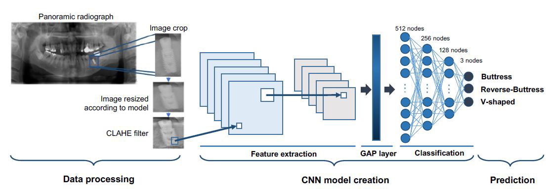
Selected radiographic images were resized according to the requirements of each model. Xception was modified to 229 × 229 × 24b, InceptionV3 to 299 × 299 × 24b, ResNet50V2, and ResNet101V2 to 224 × 224 × 24b. In addition, a contrast-limited adaptive histogram equalization (CLAHE) filter was applied to increase the image visibility.

Next, a ten-fold cross-validation procedure was performed. Cross-sampling is a resampling procedure used to evaluate machine learning models with limited dataset, and aims to overcome deviations in the datasets used to train a deep learning model for image classification.⁹ The datasets were randomly split into ten partitions, with one part used as the testing dataset and the other nine parts used as the training dataset. Care was taken to ensure that the training and test data did not contain samples from the same tooth or patient. Data augmentation was used to increase the number and diversity of the images. This was randomly performed with a vertical flap of the image, rotation of -10 degrees to +10 degrees, shift from -10% to +10%, and distortion of 10%.

5. The Architecture of the Deep CNN Algorithm

Various neural network models are now readily available from the Keras in TensorFlow. In this study, Xception, ResNet50V2, ResNet101V2, and InceptionV3 were selected. A GlobalAveragePooling2D layer and four dense layers were added at the end of each model to visualize the model and classification. The output numbers of the four dense layers were 512, 256, 128, and 3, and the activation mode was set to ReLU for the upper 3 and Softmax for the lowest. All the dense layers were connected to a fully connected layer. The model architectures and hyperparameters were optimized using a randomized search. Fig. 1 shows the overall flow starting from image preprocessing and the schematic structure of the model.

Fig. 1.

The overall scheme of the pre-trained convolution neural network. Image preprocessing was done following the acquirements of each model and applying a Contrast Limited Adapted Histogram equalization (CLAHE) filter for enhanced visibility.

The dataset classification according to the type of implant thread followed by a 10-fold cross-validation is shown in Table 2.

The algorithms were run on an Intel^® Core^TM i7-8750H CPU @ 2.20GHz, with a RAM of 16GB, on a 64-bit operating system, and using an NVIDIA GeForce GTX 1050 Ti GPU.

Categorical cross-entropy was used as the loss function for learning, and RMSprop was used as the optimizer. The learning process was conducted over 100 epochs. The learning rate was set to 2 × 10^-5 and the batch size was set to 32.

6. Statistical Analysis

The accuracy and area under the curve (AUC, calculated from receiver operating characteristic (ROC) analysis) of each of the four models were obtained. Based on the diagnostic performance of each model from each fold, the accuracy and loss of each model were compared using the Mann-Whitney U Test, and the AUC values ​​were compared using McNemar’s chi-square analysis. The level of significance was set at p < .05.

Ⅲ. Results

1. Accuracy and Loss in Training and Validation Datasets

Fig. 2 shows the average accuracy and loss plots of the training process for each model. For the training dataset, all four models exhibited convergence of accuracy and loss.

Fig. 2.

The average accuracy and loss during 100 epochs from the 10-fold cross-validation procedure. The X-axis represents the number of learning epochs, and the Y-axis represents the accuracy and loss respectively. The red line indicates the training dataset and blue the test dataset.

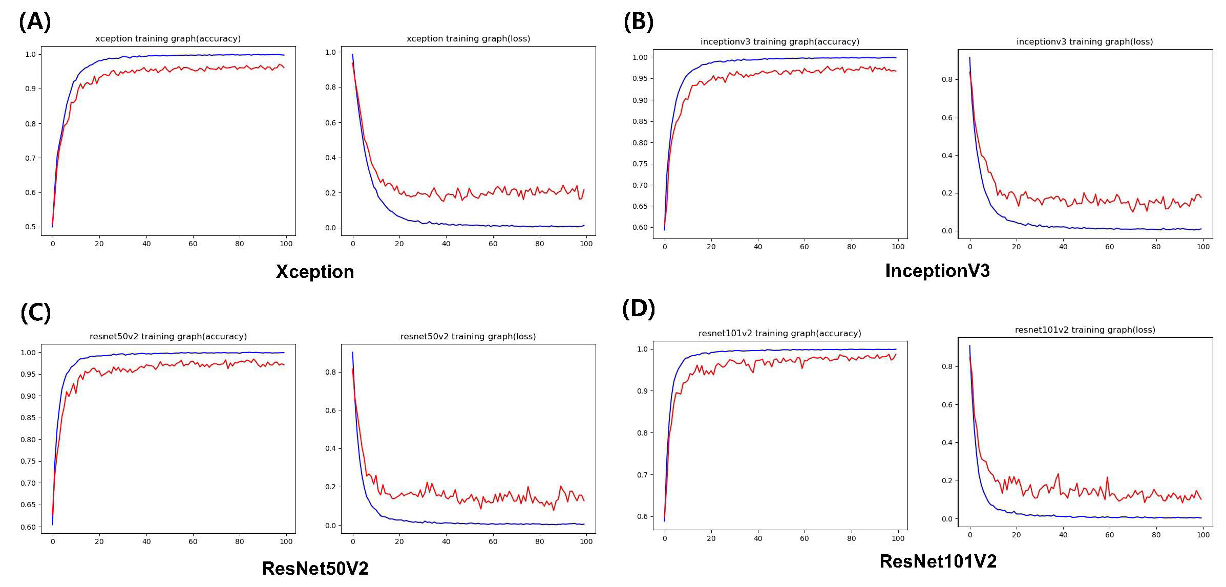
According to the results from the validation dataset, the accuracy of ResNet101V2 was the highest at 98%, and it exhibited the lowest loss. Xception exhibited an accuracy of 96% and the lowest loss was 0.003973%. Each model achieved an AUC of > 0.96, 0.961 (95% CI 0.952–0.970) with Xception, 0.973 (95% CI 0.966-0.980) with InceptionV3, an AUC of 0.980 (95% CI 0.974-0.988) with ResNet50V2, and 0.983 (95% CI 0.975-0.992) respectively. When comparing the accuracy between the different placement sites, the accuracy was higher in the posterior region than in the anterior area in all four models. ResNet50V2 demonstrates an accuracy of > 85% in all areas. The diagnostic performance measures for determining the implant type for each deep learning model are presented in Table 3. The p-value between the four models considering accuracy was 0.0426, loss was 0.5579, and 0.0021 for AUC. Multiclass classification confusion matrices were drawn from the results, as shown in Fig. 3.

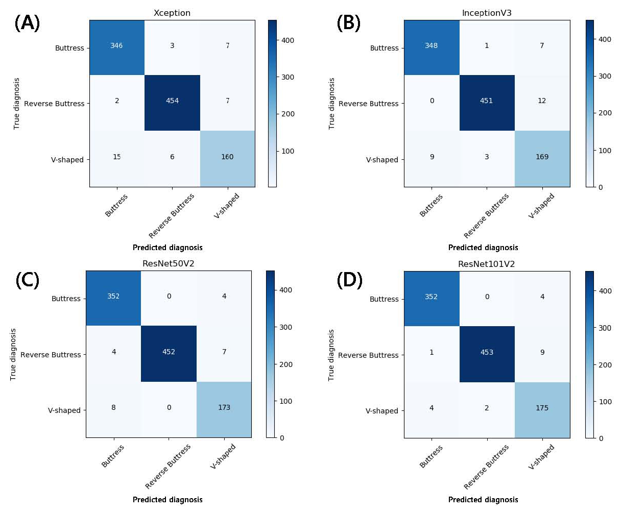
Fig. 3.

Multiclass classification confusion matrix using (A) Xception, (B) Inception, (C) ResNet50V2, (D) ResNet101V2 without normalization. The diagonal elements represent the number of points where the predicted label matches the actual label, while the non-diagonal elements show the incorrect detections made by the classifier. The higher the diagonal value and the darker the shade of blue, the more accurate the diagnosis.

2. Visualization of Model Classification

Deep CNNs demonstrate high predictions, yet do not explain how these predictions are made. Thus, to compare model performance based on human perception and add interpretability to the model, Grad-CAM was applied to visualize class activation maps (CAM) on the implant threads shown in the radiographic image. A Class Activation Map can be drawn using a Global Average Pooling Layer.¹⁰

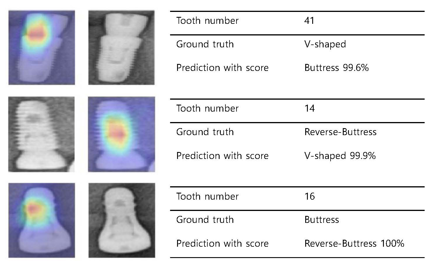
When the CNN visualizes the extracted features, most CAMs highlight the implant surface where the threads are present. However, some CAMs show a response in the healing abutment or the connection between the healing abutment and the fixture, rather than the threaded portion of the implant. Examples of the prediction accuracy and CAM obtained from ResNet101V2, which exhibited the highest accuracy among the four models, are shown in Fig. 4. A failure analysis of the incorrectly classified cases is shown in Fig. 5.

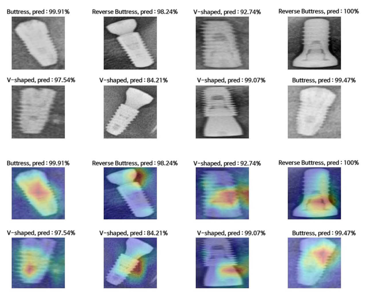
Fig. 4.

Radiograph examples and activation maps. (Top two rows) Examples of predictions obtained from ResNet101V2 according to implant thread shape. (Lower two rows) Class Activation Map (CAM)s drawn from the Global Average Pooling (GAP) layer. The model generally focuses on the implant threads, but in some cases, it highlights the connection area.

Fig. 5.

Failure analysis of incorrectly classified cases. Heat maps are visible on the healing abutment or the connection area instead of the threaded portion of the implant, implying overfitting.

Ⅳ. Discussion

Research to identify various dental implant systems by employing artificial intelligence algorithms is actively underway. One report showed an accuracy of 93-98% in classifying four types of implants using 801 periapical radiographs and five pre-trained CNN models,¹¹ while another reported an accuracy of 86–93% in distinguishing 11 implant types among 8859 panoramic images using five CNN models.¹² These attempts used deep learning algorithms, a form of data-driven AI built on a bottom-up concept that trains mathematical models with an image database.¹³ The neural networks used in these studies, each using small or large datasets, implement a learning process that adapts image features from the input dataset and performs object detection and classification. The diagnostic accuracies of these studies are relatively high; however, they fail to demonstrate the process by which the actual decision was made. Furthermore, the process cannot be interpreted in a medically acknowledged context and fails to provide interpretability and transparency.¹⁴ To add interpretability to the algorithm, a knowledge-based AI approach can be added to the deep learning process. Dental clinicians classify implant systems using a top-down method by recognizing the distinguishing features of the implant shown in the radiograph, such as thread shape, and adding other features to identify the fittest candidate; this logic was expected to be conjugated to the AI classification hierarchy. Therefore, this study was a trial application to construct a model that distinguishes the critical features of an implant system, and in further studies, synthesizes the features to predict a specific implant system or at least present a list of possible systems, rather than specifically predicting all known implant systems. By using this logic, the model is not required to learn every single implant system available in the market; rather, through a less exhausting learning procedure of certain features conjugated with a premade backup of a database of possible implant systems, it can predict the most eligible candidate in a clinician’s decision-making process.

The structure of a deep CNN algorithm is critical for achieving superior AI performance. The pre-trained deep learning models used in this study were Xception, ResNet50V2, ResNet101V2, and InceptionV3, all of which were provided by Keras. Pre-trained models have the advantage of requiring less training time and data.¹⁵ However, reports suggest that pre-trained models accelerate convergence early in training but do not necessarily provide regularization or improve the final target task accuracy.¹⁶ All four models showed an accuracy of over 92%, indicating that performance may be improved by fine-tuning and additional transfer learning techniques.¹⁷

The size of the model varied depending on the number of nodes and weights of each model, and the accuracy varied depending on the configuration of the layers. These four models are in the size range of 88–171 MB but have been reported to show over 0.93 in top-5 accuracy.¹⁸ Owing to limitations in computing power, these four models were chosen among many others for this study. According to Sunny et al., insufficient computational resources in data processing have become obstacles, constraining the efficiency of AI.¹⁹ Upgrades in computing power are expected to result in accelerated AI performance.

The number of images prepared in this study was more than 10,000 for each group after data augmentation, and a 10-fold cross-validation was applied because of the limited dataset; however, the quantity of the training dataset used in this study may still be considered insufficient. Although deep CNN architectures are highly useful in cases where the available training sets are limited, small datasets can be a bottleneck for the further advancement of computer-aided detection.²⁰ For high AI performance, the use of a high-quality training dataset is crucial, and this can be achieved by implementing high-quality, well-annotated datasets.

Image filtering is implemented to increase the visibility of images used for medical diagnosis. Attia et al. compared the effect on prediction accuracy of three image filtering methods: Imadjust, Histogram Equalization, and Contrast Limited Adaptive Histogram Equalization (CLAHE). When image enhancement was applied to a chest X-ray and compared using image quality measurement techniques, such as Mean Square Error (MSE) and Peak Signal-to-Noise Ratio (PSNR), CLAHE proved to be the most effective.²¹ Thus, CLAHE was chosen as the filtering method for this study. This is expected to compensate for the limitations caused by downscaling the resolution of radiographic images to some extent, since downscaling was unavoidable due to limitations in computational costs and operating space.²² However, other methods can be expected to be applied in future studies for enhanced results.

Overcoming the black-box nature of deep learning algorithms and ensuring reasonable interpretation to reflect the rationale behind predictions is a challenge for the application of AI in dentistry. Class activation maps highlight the areas focused on prediction, strengthening the model’s reliability through visualization capacity. Zhou et al. reported that adding a Global Average Pooling (GAP) layer to the last layer of a neural network instead of a flattening layer can build a generic localizable deep representation that exposes the implicit attention of CNNs on an image.¹⁰ Most CAMs highlight the implant surface where threads are present; however, some localize the healing abutment or connection area instead of the threaded portion of the implant. This is presumably because when the CNN clusters implant types according to the thread shape, it focuses on areas other than the implant surface, implying overfitting of the model. More data is required to ensure increased accuracy and transparency.

Among the four models, ResNet101V2 exhibited the highest accuracy in the validation dataset, while all models showed lower accuracy at the anterior than at the posterior sites. This could be the result of the overlap of various structures in the anterior area, along with the increased blurring and magnification of this area, which is often observed in panoramic images. Fluctuations are observed in the loss plot during the learning process. This, in addition to the unfavorable localization of CAMs mentioned above, reflects the likelihood of overfitting. Overfitting in this study can be explained by insufficient data and image distortion. Data shortages occurred because the types of implants were biased towards a particular model. Clinicians show preferences in selecting implants;²³ thus, it is difficult to collect an equal number of cases from various systems. Among the eight types of implant systems investigated in this study, dentin implants accounted for 35% of the total number of implants. The image distortion in panoramic radiographs was greater than that in periapical images. Therefore, the thread shape of the implant is more likely to be distorted, making it difficult for the AI to recognize. The distortion rate was highest in the maxillary incisor area and lowest in the mandibular second premolar and first molar areas, regardless of the patient’s head position.²⁴ This coincides with the accuracy according to the implant site, and the lower accuracy rate in the anterior portion is expected to contribute to overfitting.

This study has notable limitations. First, the sample size used in this study was relatively small compared with other CNN-related studies. This is because the radiographic images were obtained from patients who underwent implant surgery at a single institution; resulting in a limited number of patients enrolled for data collection. The number of images prepared in this study was multiplied through data augmentation, and 10-fold cross-validation was used; however, the quantity of the training dataset used in this study may still be considered insufficient. Although deep CNN algorithms with pre-trained weights are highly useful in cases where available training sets are limited, small datasets can be a bottleneck for the further advancement of computer-aided detection.²⁰ For high AI performance, the use of a high-quality training dataset is crucial, which can be achieved by implementing high-quality, well-annotated datasets. Second, data homogeneity was present because the data were collected from a single institution. Although pre-trained deep CNN models using large image datasets are effective for general image classification because of their pre-trained weights, the possibility of overfitting cannot be excluded when using a small dataset with a singular character originating from a limited data source. External validation is required to confirm that multicenter studies are necessary to increase the classification accuracy. With further improvements made using additional refined data, the fine-tuning of the models can be expected to be optimized to distinguish among the various implants used worldwide. Finally, among the various implant design features, only the thread shape was considered; this was further divided into three categories. However, other features of implant design can be subdivided into numerous other categories. Implant systems vary in fixture shape (straight, tapered, or conical), emergence, screw, or abutment design. Such variables can be implemented to advance the accurate classification and proposal of system candidates.

Ⅴ. Conclusion

In conclusion, the CNN models used in this study could accurately classify implants in all areas of the oral cavity according to the thread shape using radiographic images. All models exhibited higher performance in the posterior area, and the overall performance was the highest when using ResNet101V2. These models can support automated implant classification in educational fields and clinics.